In this context, we would attribute gaps in the data to some procedural failure, defective sensors, patients in a clinical trial not showing up, websites being down etc., but often “missingness” is an intrinsic feature of the data source at hand. This is the case for many transaction based metrics:

• the price of a consumer good or a stock is only reported when a sale takes place,
• the inventory of a warehouse is updated only when items are received or going out,
• and, of course, the number of businesses only changes when companies start up or go out of business.

Regardless of whether the reason is due to failure or or to plan, in many applications we have to somehow impute the missing items for those times where no data is available.

Let’s have a look at some simulated data to see how this might work. For concreteness we assume hourly time series of sales and prices of some products on a website or in a store.

library(tidyverse)
library(ggplot2)

# Parameters of the simulated data

set.seed(1756) 
NProd = 20000 # number of articles 
NTime = 100 # number of times , e.g. hours
AvSales = sort(runif(NProd, 0.7, 5)) # average hourly sales (lowest first)
NPriceCh = sample(6:12, NProd, replace = TRUE)# number of price changes  
StartPrice = runif(NProd, 1, 10) # average price of each article
PriceSteps <- c(-(6:1), 1:6)*0.05

createData <- function(art) {
  ## simulate prices and sales
    stepPrice <- rep(0, NTime)
    stepPrice[sample(seq(1, NTime, by = 3), NPriceCh[art])] <-
      sample(PriceSteps, NPriceCh[art], replace = TRUE)
    
    tibble(
      sales = rpois(NTime, AvSales[art]),
      article = paste("Prod", 1000000L + art),
      price = round(StartPrice[art] *
                      pmax(0.5, 1 + cumsum(stepPrice)), 2),
      time = 1:NTime)
}
      
fulldat <- bind_rows(lapply(1:NProd, createData))

showdat <- filter(fulldat, article =="Prod 1000001")
head(showdat)

## # A tibble: 6 × 4
##   sales      article price  time
##   <int>        <chr> <dbl> <int>
## 1     2 Prod 1000001  7.93     1
## 2     0 Prod 1000001  7.93     2
## 3     0 Prod 1000001  7.93     3
## 4     1 Prod 1000001  7.93     4
## 5     0 Prod 1000001  7.93     5
## 6     1 Prod 1000001  7.93     6

This is the full simulated data, including all 0 sales. In a typical sales transaction system, all the red points in the graphs below would not appear.

gg1 <- ggplot(data = showdat, 
              aes(x = time, y = sales)) + 
  geom_step(color = "grey" , size =1.5) + 
  geom_point(aes(color = (sales == 0))) +
  scale_color_manual(values = c("TRUE" = "darkred", "FALSE"= NA), 
                     guide =FALSE) 
gg1 

Correspondingly, we would also be missing the displayed price information for all time periods where no sale was performed.

gg2 <- ggplot(data = showdat, 
              aes(x = time, y = price)) + 
  geom_step(color = "grey", size =1.5) + 
  geom_point(aes(color = (sales == 0))) +
  scale_color_manual(values = c("TRUE" ="grey", "FALSE"= NA), 
                     guide =FALSE)
gg2

So, the simulated data set for our demonstration is obtained by removing the 0 sales:

dat <- fulldat %>% filter(sales>0)
head(dat)

## # A tibble: 6 × 4
##   sales      article price  time
##   <int>        <chr> <dbl> <int>
## 1     2 Prod 1000001  7.93     1
## 2     1 Prod 1000001  7.93     4
## 3     1 Prod 1000001  7.93     6
## 4     1 Prod 1000001  7.93     8
## 5     1 Prod 1000001  6.74    11
## 6     1 Prod 1000001  6.74    12

Given such a data set, what prices would we impute at times 2, 3, 5, 7, 9, etc.? Since here we know the mechanism leading to the missing data, a natural procedure would be to use the last valid price. This is sometimes called “last observation carried forward”, or “locf” for short. There is also “nocb” and many other methods whose relative merits, drawbacks and biases you can learn a lot about by typing these keywords into Google.

All that I am going to say here: When running such a procedure, you should have some notion about the mechanisms generating the data and the reasons for missingness. For instance, if we are looking at retail prices at a traditional store around the corner, assuming that the last price from a few hours ago is still valid, seems reasonable enough. This may have to be reconsidered if our data gap is at the beginning or the end of a known promotional period, or for an online store, where prices may be changed more dynamically, or if the gap spans a longer period of time etc.

Not imputing your data, for example ignoring situations where no sale took place in a business drivers or attribution analysis, can be a serious mistake and can strongly bias the measurement of these drivers.

This may be the topic of another article. For now, I want to look at the technical implementation of the locf / nocb procedure, which is at the basis of most other procedures. We start by sorting (assuming we don’t know if the data is sorted) and add the information on the data gaps

# arrange by hours and calculate lead and lag
dat <- dat %>% ungroup() %>%
  arrange(article, time) %>%
  group_by(article) %>%
  mutate( timeafter = lead(time, 1),
          timebefore = lag(time, 1),
          timeafter = ifelse(is.na(timeafter), time + 1, timeafter),
          timebefore = ifelse(is.na(timebefore), time - 1, timebefore) )

## Time difference of 3.595551 secs

head(dat) 

## Source: local data frame [6 x 6]
## Groups: article [1]
## 
##   sales      article price  time timeafter timebefore
##   <int>        <chr> <dbl> <int>     <dbl>      <dbl>
## 1     2 Prod 1000001  7.93     1         4          0
## 2     1 Prod 1000001  7.93     4         6          1
## 3     1 Prod 1000001  7.93     6         8          4
## 4     1 Prod 1000001  7.93     8        11          6
## 5     1 Prod 1000001  6.74    11        12          8
## 6     1 Prod 1000001  6.74    12        17         11

We now create a template dataset datImp of what data should really be present. To create the expected data, we are building the square of all articles with all times. For simplicity, we decide not to deal with imputation before the first or after the last observation. The variable “One” is only there to prevent dplyr from complaining that it does not find any common variables to join.

# max time and min time per article
lims <- dat %>% group_by(article) %>%
                summarise( mint = min(time),
                           maxt = max(time),
                           One = 1L)

# expected sales  hours X articles
datImp <- lims %>%
  left_join(data_frame(time = 1:NTime,  One = 1L)) %>%
  filter(time >= mint, time <= maxt) %>%
  select(article, time)

## Time difference of 0.7684343 secs

head(datImp) 

## # A tibble: 6 × 2
##        article  time
##          <chr> <int>
## 1 Prod 1000001     1
## 2 Prod 1000001     2
## 3 Prod 1000001     3
## 4 Prod 1000001     4
## 5 Prod 1000001     5
## 6 Prod 1000001     6

You could now join the original data frame dat to the data frame of expected data and obtain the data set where missing data is marked as NA. This is the situation that most R-packages for imputation (e.g. tidyr , zoo , padr ) take as a starting point.
In the present data set, where missingness is really absence of data, I have found that the following lines, where each " last observation " is just repeated as often aa is required to fill the gap, work amazingly well also on large data sets.

# add next hour and last hour info
datImp <- datImp %>%
  mutate(lasttime = rep(dat$time, dat$timeafter - dat$time),
         nexttime = rep(dat$time, dat$time - dat$timebefore),
         # lastart = rep(dat$art,dat$timeafter - dat$time),
         lastprice = rep(dat$price, dat$timeafter - dat$time),
         nextprice = rep(dat$price, dat$time - dat$timebefore))

## Time difference of 0.1430166 secs

head(datImp) 

## # A tibble: 6 × 6
##        article  time lasttime nexttime lastprice nextprice
##          <chr> <int>    <int>    <int>     <dbl>     <dbl>
## 1 Prod 1000001     1        1        1      7.93      7.93
## 2 Prod 1000001     2        1        4      7.93      7.93
## 3 Prod 1000001     3        1        4      7.93      7.93
## 4 Prod 1000001     4        4        4      7.93      7.93
## 5 Prod 1000001     5        4        6      7.93      7.93
## 6 Prod 1000001     6        6        6      7.93      7.93

In my applications, this simple procedure has beaten all implementations I have tried in SQL-dialects or with special purpose packages. Of course, before using this in any kind of production, one should test thoroughly.

datComp <- datImp %>% left_join(dat)

# must all be true etc. etc.
table(datComp$lastprice == datComp$price)
table(datComp$time <= datComp$nexttime)
table(datComp$time >= datComp$lasttime)

Since we started with the full simulated data in the first place, let’s wrap up this article with that comparison:

fulldat <- fulldat %>% left_join(datImp)

showdat <- filter(fulldat, article =="Prod 1000001")

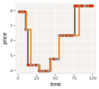
gg3 <- ggplot(data = showdat, 
              aes(x = time, y = price)) + 
  geom_step(color = "grey", size =1.5) + 
  geom_step(data = showdat, aes(x = time, y = lastprice), 
            color = "orange",
            size =1.5) +
  geom_point(aes(color = (sales == 0))) +
  scale_color_manual(values = c("TRUE" ="darkred", "FALSE"=  "grey" ), 
                     guide =FALSE) 
gg3 

As you can see the technical procedure works nicely. Unsurprisingly, differences occur when prices were changed while no sale was made. So, in a real situation it will still be useful to add external knowledge about the price setting to improve the quality of the imputation further.